Open FreeCAD software. (FreeCAD version 0.19 was used but any vrsion is suitable)

Files :

Introduction
This document presents how to create a simple project in CAPITOLE-RCS. The model used is a simple sphere with a radius of 200 mm. The Monostatic RCS calculation will be computed at a frequency of 2.5GHz on a cut in conical coordinate system at elevation 0° and from -90° to 90° on azimut angle with 37 points.

1. Creation of the model
Open FreeCAD software. (FreeCAD version 0.19 was used but any version is suitable)
Click on « New » to create a new project
Switch the workbench to « Part »

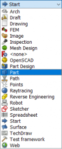
Click on the « sphere » button
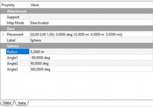
Select the object « Sphere » on the treeview
Change the Radius to « 0.2 m »

Save the Project
In « File » Menu, click on « Export »
Select « STEP » file Format.
For exemple : sphere200mm.step

2. Define simulation parameters
Execute CAPITOLE-RCS (CAPITOLE-RCS version 2.3.9 is used in this document)

Click on Blue Menu, then « Import » and « CAD File »

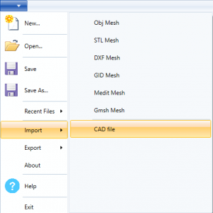
Select File Type « STEP » and select the file sphere200mm.step
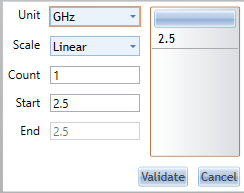
In Project Panel, define the frequency
Click on the button
Enter a single Frequency of 2.5 Ghz

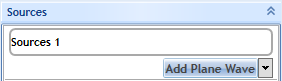
Create a Source

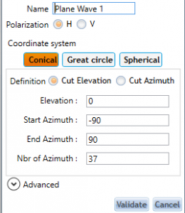
Click on PlaneWave for this source

Create a conical cut at Elevation 0° and Azimut from -90 to 90° with 37 points.
Polarization is Horizontal.

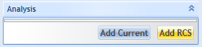
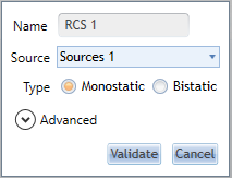
Create an RCS analysis :

In Geometry Menu, click on « Generate Mesh »
Leave the default mesh size, which is at λ/10

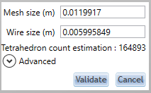
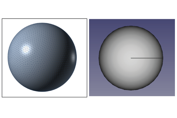
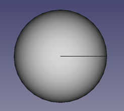
The mesh model will be created.

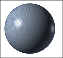
Figure 1 – Sphere mesh model

In the Solver Menu, click on « Run »

Leave the default Solver « Full »

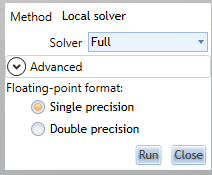
Click « Run »
The calcul will start.
The process uses 1.9 GB of RAM memory
The calculation duration is 36 s on a Laptop with Intel Core i7-7700HQ CPU
When it is finished, in the menu « Tools » click on « POSTPRO»

The project « sphere200mm » will be opened automatically in POSTPRO3D.
Click on the right of the result « RCS 1 » on the green plus sign to display the monostatic RCS curve depending on the azimuth angle.
A curve can be observed. The value of about -9dBm² is almost constant over the azimut which is close to the theoretical estimation of RCS of a sphere in optical region.
σ= πr^2

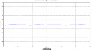
Figure 2 – Monostatic RCS of a sphere