
Introduction
This document presents simulation results from CAPITOLE-RCS on simple shapes. The monostatic RCS is calculated and compared to measured data publish in the following article : A.C. Woo, H.T.G. Wang, M.J Schuh and M.L Sanders « Benchmark Radar Targets for the Validation of Computational Electromagnetics Programs » IEEE Antennas and Propagation Magazine, Vol. 35, No. 1, February 1993. Theses models are intended for validation and benchmarking of Electromagnetic Simulation softwares. All simulations with CAPITOLE-RCS software was made on a Windows 10 laptop with Intel core i7 CPU and 16 Gb of RAM memory
1. NASA Metallic Almond
- Model :
The NASA almond is actually not a simple shape. It is defined by mathematical equations to form a surface with almond shape. This model is very intersting to study RCS because it highligts a large dynamic on RCS value. The mesh should be refined on the tip and the bottom to keep a good accuray on the results.
The total length is 0.25 m (9.936 inches)
- Simulation parameters :
The Monostatic RCS is computed at 3 frequencies : 1.19, 7 and 9.92 GHz
For both Vertical and Horizontal polarization
The RCS is plotted in dBm2 as function of azimuth angle from 0 to 180°. Zero degrees azimuth corresponds to incidence on the tip. The elevation angle is zero.
- Solver :
Method of Moment method was used with MSCBD solver and EFIE equations.
| 1.19 GHz | 7 GHz | 9.92 GHz | |
| Mesh size | Lambda/40 | Lambda/15 | Lambda/15 |
| Number of unknowns | 3 546 | 17 262 | 34 692 |
| Total time | 2 seconds | 17 seconds | 57 seconds |
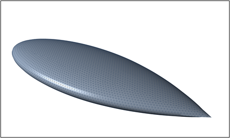
Figure 1 – NASA Almond mesh model
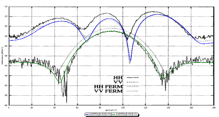
Figure 2 NASA Almond RCS @1.19GHz CAPITOLE-RCS vs measurement
2. Metallic Simple Ogive
- Model :
The model was created from the analytic expression to create a curve and revolved to create a surface. The total length is 0.254 m (10 inches)
- Simulation parameters :
The Monostatic RCS is computed at 2 frequencies : 1.18 and 9 GHz
For both Vertical and Horizontal polarization
The RCS is plotted in dBm2 as function of azimuth angle from 0 to 180°. Zero degrees azimuth corresponds to incidence on the tip. The elevation angle is zero.
- Solver :
Method of Moment method was used with MSCBD solver and EFIE equations.
| 1.18 GHz | 9 GHz | |
| Mesh size | Lambda/50 | Lambda/20 |
| Number of unknowns | 3 648 | 34 968 |
| Total time | 1 second | 1 min 12 s |
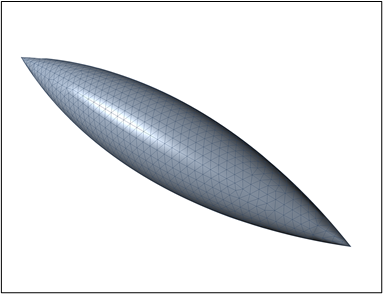
Figure 3 – Metallic Simple Ogive mesh model
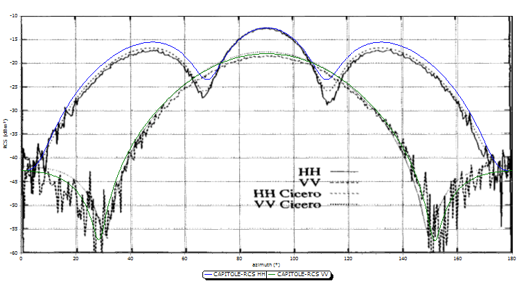
Figure 3 – Metallic Simple Ogive RCS @1.18GHz CAPITOLE-RCS vs measurement
3. Metallic Double Ogive
- Model :
The model was created from the analytic expression to create a curve and revolved to create a surface.
The total length is 0.191 m (7.5 inches)
- Simulation parameters :
The Monostatic RCS is computed at 2 frequencies : 1.57 and 9 GHz
For both Vertical and Horizontal polarization
The RCS is plotted in dBm2 as function of azimuth angle from 0 to 180°. The elevation angle is zero.
- Solver :
Method of Moment method was used with MSCBD solver and EFIE equations.
| 1.57 GHz | 9 GHz | |
| Mesh size | Lambda/40 | Lambda/15 |
| Number of unknowns | 3 288 | 15 096 |
| Total time | 1 second | 13 seconds |
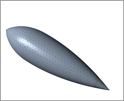
Figure 5 – Metallic Double Ogive mesh model
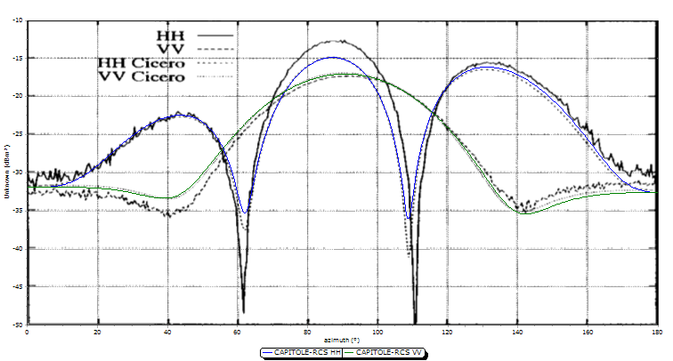
Figure 6 – Metallic Double Ogive RCS @1.57GHz CAPITOLE-RCS vs measurement
4. Metallic Cone-Sphere
- Model :
The model was created from the analytic expression to create a curve and revolved to create a surface.
The total length is 0.689 m (27.127 inches)
- Simulation parameters :
The Monostatic RCS is computed at 2 frequencies : 869 MHz and 9 GHz
For both Vertical and Horizontal polarization
The RCS is plotted in dBm2 as function of azimuth angle from -180 to 0°. -180 degrees azimuth corresponds to incidence on the tip. The elevation angle is zero.
- Solver :
Method of Moment method was used and EFIE equations.
MSCBD solver for 869 MHz case and MLACA for 9 GHz case.
The MLACA solver is more accurate for low level RCS, particularly for 9 GHz conesphere in HH polarization.
| 869 MHz | 9 GHz | |
| Mesh size | Lambda/40 | Lambda/20 |
| Number of unknowns | 8 664 | 227 793 |
| Total time | 12 seconds | 3h 11min
*on a 48 cores server |
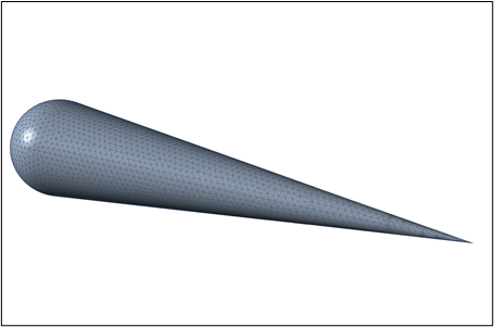
Figure 7 – Cone-Sphere mesh model
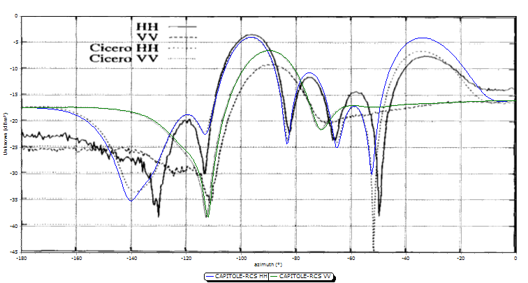
Figure 8 – Metallic Cone-Sphere RCS @869MHz CAPITOLE-RCS vs measurement
5. Metallic Cone-Sphere with Gap
- Model :
The model was created from the analytic expression to create a curve and revolved to create a surface.
The total length is 0.689 m (27.127 inches)
- Simulation parameters :
The Monostatic RCS is computed at 2 frequencies : 869 MHz and 9 GHz
For both Vertical and Horizontal polarization
The RCS is plotted in dBm2 as function of azimuth angle from -180 to 0°. -180° degrees azimuth corresponds to incidence on the tip. The elevation angle is zero.
- Solver :
Method of Moment method was used with MSCBD solver and EFIE equations.
| 869 MHz | 9 GHz | |
| Mesh size | Lambda/40 | Lambda/15 |
| Number of unknowns | 8 952 | 131 508 |
| Total time | 13 seconds | 7 min 26 s |
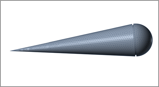
Figure 9 – Cone-Sphere with gap mesh model
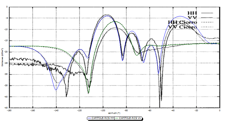
Figure 9 – Metallic Cone-Sphere with gap RCS @869MHz CAPITOLE-RCS vs measurement