RCS of a sphere as function of frequency
Files:
Introduction
This document presents a RCS simulation of a sphere with CAPITOLE-RCS. The model used is a simple sphere with a radius of 0.2 m. The Monostatic RCS calculation will be computed in one direction and for a frequency sweep from 10 MHz to 8 GHz.
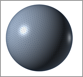
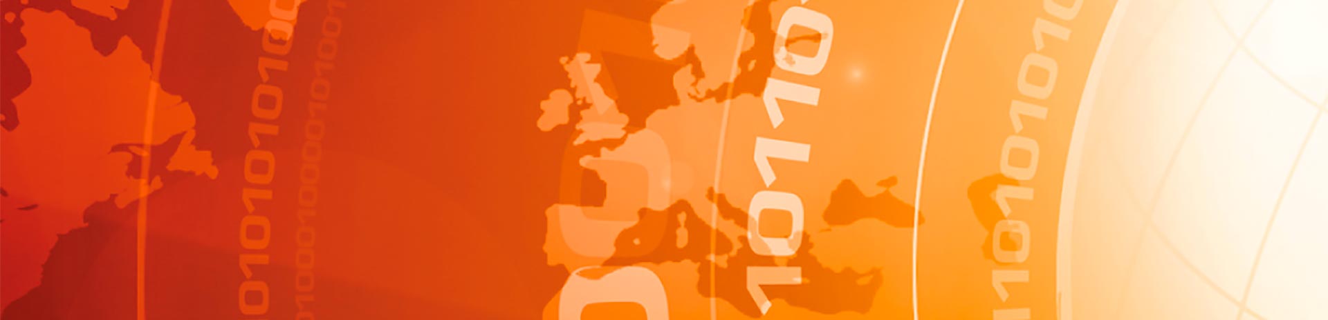
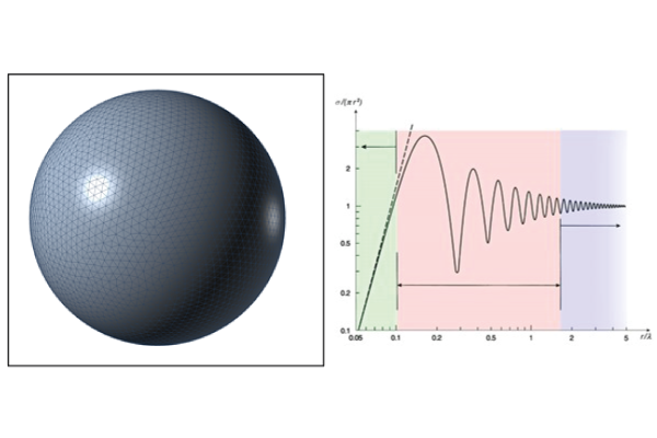
Figure 1 – Sphere mesh model
1 – Geometry model
Use the sphere model described in « Getting Started with CAPITOLE-RCS » example.
The file is sphere200mm.step
2 – Simulation strategy
In this case, the frequency range is very large, from 10 MHz to 8 GHz.
Because CAPITOLE-RCS is based on a frequency domain method, it is not advised to use a single mesh for the whole frequency sweep. Instead, you should create several CAPITOLE-RCS projects for a sub-band of frequency range and using a mesh model suitable for this frequency range. Keep in mind that the mesh size should always λ/10 or less at the higher frequency.
| File name | Frequency Range | # of triangles | Mesh size | Solver | Calculation Time |
| sphere100.h5 | 10-100 MHz | 1380 | λ/1026 – λ/102 | Full | 3s |
| sphere1000.h5 | 100-1000 MHz | 1380 | λ/102 – λ/10 | Full | 29s |
| Sphere2000.h5 | 1000-2000 MHz | 5426 | λ/20 – λ/10 | MLACA | 1min42s |
| Sphere3000.h5 | 2000-3000 MHz | 12194 | λ/15 – λ/10 | MLACA | 4min22s |
| Sphere4000.h5 | 3000-4000 MHz | 21664 | λ/13 – λ/10 | MLACA | 7min6s |
| Sphere5000.h5 | 4000-5000 MHz | 33858 | λ/13 – λ/10 | MLACA | 11Min26s |
| Sphere8000.h5 | 5000-8000 MHz | 136 264 | λ/16 – λ/10 | MLACA | 1h15min18s |
The MLACA solver is the most efficient, because it uses a compression of impedance matrix. But at low frequency, the electric mesh size become smaller and it is impossible to use MLACA solver when mesh size is under λ/100, instead it is possible to use the Full solver.
All simulations were executed on a DELL server PowerEdge R920 with 4 CPUs Intel Xeon E7-8857 v2 3.0 GHz 12 cores, 512Go of memory
All projects file can be opened with POSTPRO3D at the same time. And a single graph can display all results.
Figure 2 – Sphere RCS as function of frequency
There are 3 regions of the RCS of a sphere. It can be observed on this graph.
The Rayleigh region, when λ>10 r
For a 0.2m sphere, it is until 150 MHz
The creeping wave effect occurs when λ=2πr
It corresponds to a frequency of 239 MHz where there is a maximum RCS.
The optical region starts when 2πr/λ>10
For a 0.2m sphere it corresponds to 2.39 GHz
Above this frequency, the RCS of the sphere is independant to the frequency and equal to :
σ= πr^2
For a 0.2m sphere, σ = -9 dBm²
And between, Rayleigh region and optical region, this is the Mie region.
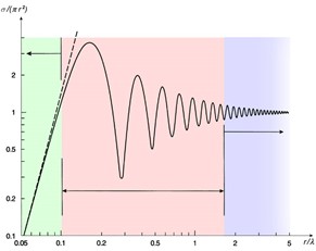
Figure 3 – Rayleigh, Mie and Optical Region
Ref 1 : https://www.radartutorial.eu/01.basics/Rayleigh-%20versus%20Mie-Scattering.en.html